As I mentioned in the last post, I have some concerns about the spin-boson model of cold fusion that are probably most easily settled via computer calculations. But before I jump into calculating something new, I want to make sure I understand the basics. So, in this post I am simply reproducing the computer calculations in Figs. 1-2 of the 2008 paper Models Relevant to Excess Heat Production in Fleischmann-Pons Experiments by Peter Hagelstein and Irfan Chaudhary. This was a fun and straightforward exercise in freshman quantum mechanics. I did not unearth any problem in the paper, nor did I expect to (at this stage). But now I have my first bit of working spin-boson code, and a bit more concrete understanding of the model. Time well spent! So without further ado…

The Hamiltonian

When analyzing a system using quantum mechanics, a Hamiltonian is kinda halfway between reality and understanding. Moving in one direction, we try to answer the question “If a hypothetical system had this Hamiltonian, how would it behave?” Moving in the other direction, we try to answer the question, “I have a real-world experimental system that I am trying to understand. Is this really its Hamiltonian?“

The answer to the second question, by the way, is always “No”, but sometimes it is “No but it’s a good enough approximation for such-and-such purpose.” We do not expect to model any real system down to the last detail (at least, not in this branch of physics!). But anyway, this post is purely about the first question, i.e. predicting a system’s behavior under the assumption that it has a certain Hamiltonian, and leaving aside the question of whether anything in this analysis is really relevant for understanding cold fusion.

So without further ado, here is the Hamiltonian for today (Eq. (1) of the paper):

where…

• are “total spin” operators that act on a collection of one or more identical two-level systems (using the term “spin” metaphorically),
• a^†,a are the creation and annihilation operators for excitations of a quantum harmonic oscillator,
• ΔE, V, and ħω₀ are three parameters with units of energy.

For example, think of ΔE as the 24MeV energy difference between two nearby deuterons (D+D) versus one helium-4 atom; ω₀ as the angular frequency of a phonon mode, a^†,a as the operators that create and annihilate phonons respectively, and V as the strength of the so-called a·cP phonon-nuclear interaction which supposedly allows nuclear transitions to excite phonons or vice-versa.

The first term of the Hamiltonian describes the fact that each D+D has ΔE more energy than helium-4, the second term accounts for the energy in the phonon vibration, and the third term is the energy that comes from the phonons and nuclei interacting with each other.

(Again, in this post we are studying the Hamiltonian while being noncommittal about how or whether it applies to cold fusion. The previous two paragraphs are describing an interpretation of this Hamiltonian, but that’s purely as a mnemonic, to make the math easier to describe and follow below. As a matter of fact, in the latest work, Prof. Hagelstein and collaborators have been proposing a slightly different interpretation of a slightly different Hamiltonian. In addition to the D+D fusion, other excited nuclear states are also involved. More on this in some future post.)

The states

In general in the spin-boson model, one writes the states as |S,m,n> where…

• S is the total spin quantum number (i.e. 2S is the [minimum] number of 2-level systems involved),
• m is the spin projection quantum number (i.e. 2m is difference between how many of the 2-level systems are in the higher-energy D-D state, versus how many are in the lower-energy helium-4 state),
• and n is the energy level quantum number for the oscillator (i.e. there are n phonons in the phonon mode of interest).

Figs. 1 and 2 of the paper assume S=½: “The models and solutions discussed here involved only a single two-level system coupled to an oscillator.” That implies two possibilities for m, i.e. ±½. Meanwhile, n can be any integer from 0 to ∞. Unfortunately it is hard to diagonalize an infinitely large matrix, but a reasonable shortcut in this case is to take a large but finite range of possible n, and just avoid doing any plots or calculations close to the edge(s) of the range.

Conserved quantities

The Hamiltonian written above cannot change S: If we start with S=½ (and we do! at least for this post), then S stays at ½, and we can forget about any other possibility.

There is a second less obvious conserved quantity here: The parity of S+m+n (i.e. whether S+m+n is an even or odd number). In other words, we cannot get transitions from |S,m,n> to |S‘,m‘,n‘> unless (S+m+n) and (S’+m’+n’) are both even or both odd. This explains why this paper (and others by the same authors) often spurn round numbers! They talk about exchanging 11 or 21 or 31 phonons, rather than 10 or 20 or 30. If m changes by 1, then n needs to change by an odd number.

Since the even and odd “sectors” exist in parallel universes, not interacting with each other, I will restrict myself to just one of the sectors at a time. This will simplify the code, the plots, and the analysis.

The computer implementation

The math and algorithm here is pretty straightforward: Fill in the entries of a Hamiltonian matrix, comput its eigenvalues and eigenvectors, making some plots, calculate some maxima and minima, etc. I will use Python, an excellent language for scientific computing. I like Python so much (vs typical alternatives) that I wrote this whole long webpage proselytizing it.

The exact code used for the plots in this post is here. Writing the code was pretty straightforward, from my perspective, so I won’t discuss any implementation details in this post. Of course, you can ask me questions about the code (and anything else) in the comments section.

The energy levels

A very easy thing to do is plot the energy levels–i.e. the eigenvalues of the H matrix–as a function of V. Here are the lowest 100 or so states in the case that ΔE=11ħω₀:

Start at the far-left (V=0): if you look closely you’ll see that there is a pair of equal-energy states, then a gap of 2ħω₀, then another pair, etc. It’s 2ħω₀ rather than ħω₀ because I am only plotting here the “S+m+n is even” sector (see the “Conserved Quantities” section above). The pair of equal-energy states correspond to (m,n) = (½ , n) and (m,n) = (-½ , n+11). Near the bottom, there are some unpaired (“nondegenerate”) states, since n cannot be negative.

Going right, the equal-energy states split apart, with one moving up and the other moving down. An obvious thing you’ll notice is the dark bands that kinda look like a Moiré pattern. The bands slope up-left and down-right, or in other words, near the top of the plot (higher n), the states bump into their neighbors at lower V than near the bottom of the plot. I know just how to quantify this:

I drew the dashed line by plotting a curve of the form y ∝ 1/x², and you see that it follows the banded pattern perfectly,   What does that mean? It means that the shift in the energy of a state depends on V√n, rather than V. And why does it depend on V√n? Recall that the interaction (third term in the Hamiltonian above) is . When this acts on |S,m,n>, we get vectors of magnitude V√n (or V√(n+1) which is similar). Keep in mind that S=½, m=±½ for present purposes, so the other expected factors like √((S-m)(S+m+1)) are all just 1. Hence V√n is the quantity that we expect to be relevant.

Next, let’s go to much larger n: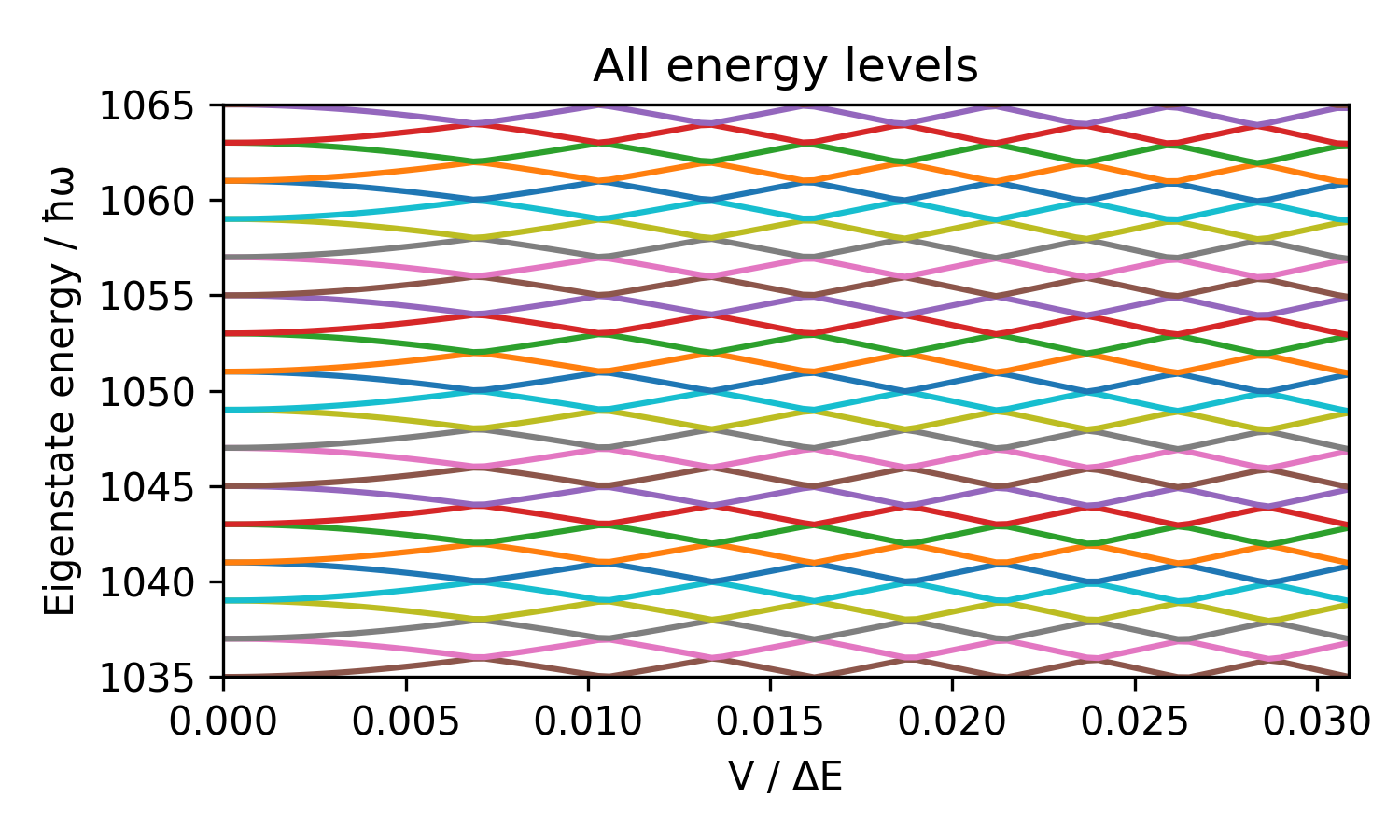

The Moiré-looking stripes appear vertical in this plot, unlike the previous plot where they were tilted and curvy. The reason is simple: √n only changes by 1% across this plot. So the bands appear vertical but aren’t quite.

Prof. Hagelstein gives an approximation for the shape of the lines in this figure:

where ≡ means “equals by definition”. In this particular example, this approximation is reasonable but not perfect:

This version is a bit easier to see:

This matches Fig. 1 in the paper, hooray! The blue graph should really be speckled with discontinuities from anticrossing, but I made it smooth by only sampling the curve away from the anticrossing regions (i.e. the values of V where the eigenvalues are curving sharply away from each other), and interpolating.

The energy eigenstates

When I wrote the equation for E_S,m,n above, I made up the notation “E_S,m,n“. It’s not written in the paper that way. And in fact, my notation is misleading in the following sense: If we take that blue eigenvalue curve from the last plot, it starts out at a certain S,m,n, but as we go rightward (larger g due to larger V), the corresponding eigenstate turns into a mixture of many different S,m,n:

The higher the value of , the more different S,m,n states get mixed into the eigenstate, until at g=1 even the 11 states I plotted add up to only 60% of the total.

The anticrossing energies

Last but not least, I calculated the anticrossing energies, i.e. the minimum energy difference between two energy eigenvalues:

(This agrees perfectly with the paper’s Fig. 2. Hooray!) The blue, orange, and green curves are respectively ΔE/(ħω₀) = 11, 21, and 31. The vertical axis is the closest that each eigenvalue curve approaches to its nearest neighbor above or below in the same parity sector (even or odd).

Why do we care about these anticrossing energies? Well, the paper’s Eq. (7) and surrounding text tells a simple story about transition rates, but I kinda think that the real story is somewhat more complicated than that. Well anyway, for present purposes, it’s just something to calculate to make sure that my code is correct.