Readers of this blog (if any exist lol) may notice that I’m on my sixth post about the lossy spin-boson model without really writing the model down. You’ll have to wait a bit longer, sorry! This post is more background.

Here I’m chronicling my progress in conceptually understanding the “lossy” part of the “lossy spin-boson model”. It is discussed most clearly in the paper “Energy Exchange in the Lossy Spin-Boson Model”.

Real and virtual states

In quantum mechanics, every system has an infinite number of energy eigenstates. Think of them as possible configurations of the system (locations of all the particles etc.).

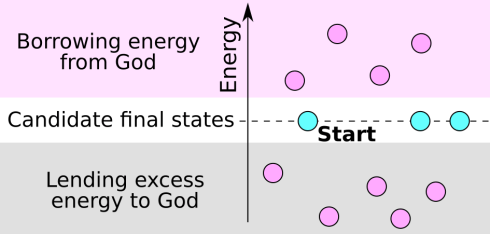
Each dot is an energy eigenstate; its vertical position is its energy. The system starts out at the dot marked “Start”.

In this diagram, I marked a bunch of energy eigenstates. The pink dots are states that the system cannot jump to without violating Conservation of Energy, while the blue dots are states that the system can jump to while satisfying Conservation of Energy. I called the blue dots “candidate final states” because they can be the endpoint of a transition.

The pink dots above the line are states that the system does not have enough energy to be in. The particles are all moving faster than at the start, etc. Thanks to Conservation of Energy, the system cannot really be in those states … but it can temporarily. I like to say that the system visits those states by “borrowing energy from God”. (This is just a humorous description, it’s nothing profound!) It’s called a “virtual state”, as opposed to a “real state” that the system can stay in permanently.

Likewise, the pink dots below the line are states with less energy than how much energy the system starts out with. The particles are all moving slower than at the start, etc. Again, the system can only temporarily be in these states. It has too much energy. I like to say jokingly that it occupies those states by “lending its excess energy to God”. Again, these are “virtual states” for the system.

As they say: “Neither a borrower nor a lender be.” The more energy that the system needs to borrow or lend to be in a state (i.e. the bigger the violation of conservation of energy), the more temporary and insignificant is the role of that state.

To be more precise about what I’m talking about here: There is a system Hamiltonian , where is the “unperturbed Hamiltonian” which describes every aspect of the system (e.g. phonon spectrum, electron excitations, etc.) except the term that describes energy coupling between nuclear transitions and phonons, while V, the “interaction term”, is just the latter. I am plotting the energy eigenstates of in that picture above. V would be drawn in as lines between various dots, in the sense that V makes it possible for the system to go from one dot to another. These transitions, both direct and indirect, can be calculated by Fermi’s golden rule or higher-order Fermi’s golden rule if V is small (perturbation theory), or otherwise by the exact time-dependent Schrodinger equation:

(So in the previous paragraphs have been using the term “energy” imprecisely, as the eigenvalue. The real energy includes V too. The real energy is always conserved, unlike the energy which can be temporarily changed.)

The cursed cancellation

In higher-order Fermi’s golden rule, the probability amplitudes have a factor called the “energy denominator”, which is positive when the intermediate state is lending energy to God, and negative when it is borrowing energy from God.

Let’s talk about this cold fusion process where we want to create a billion phonons and fuse two deuterons into a helium-4. If you create the billion phonons first, and fuse the deuterons at the end, then the intermediate states are borrowing energy from God. If you fuse the deuterons first, then create the billion phonons afterwards, then the intermediate states are lending energy to God. If you create half the phonons, then fuse the deuterons, then create the other half, you get some of each. (Note: I am oversimplifying. The transition is actually a more complicated dance, where the deuterons have to repeatedly fuse and un-fuse, etc.)

Anyway, for transition paths where there are an odd number of intermediate states that borrow energy from God, then the energy denominators collectively give a minus sign to its term in the transition amplitude. Otherwise, they give a plus sign. Out of the many paths that the transition can take, about half have an odd numbers of borrowers, and the other half have an even number. So when we add up all the amplitudes, we get “cursed cancellations”.

Remember, since we want to explain cold fusion, we were hoping that the total transition rate would be high. And if we look at the amplitude from any given transition path, it is actually impressively large (according to the authors). But, when we add up the amplitudes of all the different paths, the final transition rate is disappointingly small, because of the cancellations!

Treating borrowers and lenders differently

Peter Hagelstein (et al.) have therefore, naturally, been looking for ways to argue that the cancellation does not really happen after all. Eventually they found one they believed in:

When losses are taken into account, they argue, you need to treat the energy-borrowing-states and the energy-lending-states differently.

They give an example in which they say you can ignore every transition path except ones that have no energy-lending intermediate states whatsoever! The energy-lending intermediate states poison every transition path they touch.

In my experience, this whole idea is highly unusual. Although banks treat borrowers and lenders differently, physicists generally do not. In gazillions of calculations in all areas of quantum mechanics and quantum field theory, you sum over virtual states, and I had never before seen any situation where the states with too much energy are treated differently than the states with too little. I couldn’t really make any sense of how this argument works.

After talking to Dr. Hagelstein, I have a better understanding of what he has in mind. I drew these two pictures:

Oversimplified picture (same as above)

More accurate picture

The second picture shows that each state has a series of higher-energy siblings. Dr Hagelstein suggested that the siblings have more and more electrons that have been promoted into higher-energy states. (If I remember right he mentioned “Vibrational coupling to electron promotion”, including even K-shell ionization. But any other excitation would also work here I guess.) The states do not have lower-energy siblings, only higher-energy siblings, because you cannot have fewer than zero promoted electrons.

Now it starts to seem reasonable why the borrowers and lenders are different. The lenders have extra paths back to blue states, by promoting an appropriate number of electrons, while the borrowers do not have anything like that.

State-level loss without system-level loss?

Then I had the following complaint:

• If these “loss paths” involving final states with promoted electrons are important enough to affect the transition probabilities, I would think that their main effect would be that these loss-related transitions would actually occur. So they would compete with the transition we were hoping for.
• Conversely, if that loss-related transition essentially never happens, then I would not expect it to have any effect on the transition rate.

Dr. Hagelstein was ready with an answer to my complaint. He said that you could in fact have losses that were important from the perspective of individual virtual states, even though at a system level, the loss process almost never happens. If I remember right, he said that if the virtual state’s decay rate is equal to some other relevant rate (I don’t remember what), then the loss process actually occurs with maximum rate. However, if the virtual state’s decay rate is much lower or much higher (paradoxically), then system-level loss becomes quite low (i.e., the loss process rarely actually happens). But the fact that the loss channel exists nevertheless alters the amplitude of the corresponding state.

Got that? Neither do I, really. But it sounds correct.

Speaking of not following the details…

The evil magic of lossy quantum mechanics

“Losses”, also called “dissipation”, are processes like friction that turn energy from other forms into undesired forms, especially into heat. In a certain sense, there are no losses in quantum mechanics. In technical terms, the Hamiltonian of the universe is unitary.

For example, when you write an equation for friction, it has an “arrow of time” right there in the equation (friction always turns kinetic energy into heat, never the other way around); but the quantum mechanical laws of the universe don’t let you do that. (At least, not in such an explicit way.) A historically famous consequence of this is the “black hole information paradox”. General Relativity seemingly proved that when stuff gets sucked into a black hole, it would turn energy into heat in an irreversible dissipation process. However, such dissipation would be incompatible with the foundations of quantum mechanics. It seemed to be a paradox. The paradox was eventually resolved following work by Juan Maldacena, Stephen Hawking and others. Quantum mechanics survived: It turns out that there is no dissipation after all.

So much for the exact laws of the universe. However, you can in fact put losses into quantum mechanics calculations as an approximation! This possibility is rarely discussed in introductory quantum mechanics courses. I know very little about it. Until I understand it better, I continue to think of it as a sort of evil magic. (I think to myself: “You’re writing down a Hamiltonian which is not Hermitian? You disgust me!“)

Anyway here’s what I do know. The concept of “losses” is really related to “aspects of the system that I am not properly modeling”. This is true in both classical and quantum physics. For example, when you model a ball falling through the air, you would normally put wind resistance as a dissipative loss term. But if you have a model that includes every single air molecule, then there is no loss term.

So, while I have not yet tried to learn how to put losses into quantum mechanics calculations, I have nothing against it in principle. And I have high confidence that Peter Hagelstein does know all about it. After all, it’s discussed in this textbook he cowrote. Therefore, I am inclined to believe the things he says about modeling losses in quantum systems, even though I haven’t tried to follow all the details.

It is especially encouraging that he says that, in recent work, he has found that he can derive the same results using lossy quantum mechanics versus a lossless system with extra degrees of freedom—just like you’d expect.